European Soccer Events Analysis with Apache Spark and Databricks

The global sports market is huge, comprising of players, teams, leagues, fan clubs, sponsors etc., and all of these entities interact in myriad ways generating enormous amount of data. Some of that data is used internally to help make better decisions, and there are number of use cases within the Media industry that utilize the same data to create better products and attract/retain viewers.

Few ways how the Sports and Media industries have started utilizing big data are:

  • Analyze on-field conditions and events (passes, player positions etc.) that lead to soccer goals, football touchdowns or baseball home runs etc.
  • Assess the win-loss percentage with different combinations of players in different on-field positions.
  • Track a sportsperson’s or team’s performance graph over the years/seasons
  • Analyze real-time viewership events and social media streams to provide targeted content, and more..

European Soccer Leagues Data

We all have a favorite sport, and mine is Soccer for its global appeal, amazing combination of skills & strategy, and the extreme fans that add extra element to the game.

In this article, we’ll see how one could use Databricks to create an end-to-end data pipeline with European Soccer games data – including facets from Data Engineering, Data Analysis and Machine Learning, to help answer business questions. We’ll utilize a dataset from Kaggle, that provides a granular view of 9,074 games, from the biggest 5 European soccer leagues: England, Spain, Germany, Italy and France, from 2011 to 2016 season.

Primary dataset is specific events from the games in chronological order, including key information like:

  • id_odsp – unique identifier of game
  • time – minute of the game
  • event_type – primary event
  • event_team – team that produced the event
  • player – name of the player involved in main event
  • shot_place – placement of the shot, 13 possible placement locations
  • shot_outcome – 4 possible outcomes
  • location – location on the pitch where the event happened, 19 possible locations
  • is_goal – binary variable if the shot resulted in a goal (own goals included)
  • And more..

Second smaller dataset includes high-level information and advanced stats with one record per game. Key attributes are “League”, “Season”, “Country”, “Home Team”, “Away Team” and various market odds.

Data Engineering

We start out by creating a ETL notebook, where the two CSV datasets are transformed and joined into a single parquet data layer, which enables us to utilize DBIO caching feature for high-performance big data queries.

Extraction

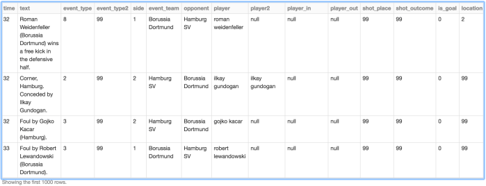
First task is to create a Dataframe schema for the larger game events dataset, so the read operation doesn’t spend time inferring it from the data. Once extracted, we’ll replace “null” values for interesting fields with data-type specific constants.

Data_Events_Extract
Game events data extraction and replace nulls

This is what the raw data (with some nulls replaced) looks like:

Data_Events_Display
Display game events data

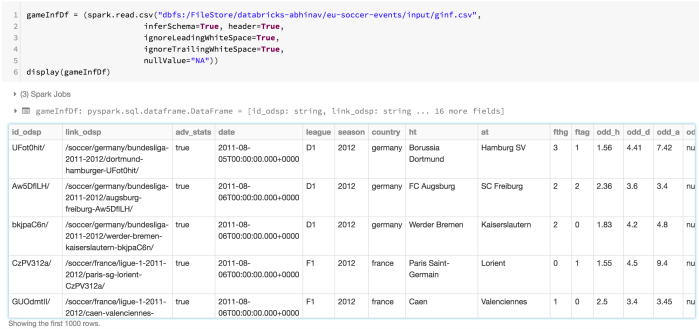
We also read the second dataset into a Dataframe, as it includes country name which we’ll use later during analysis.

Data_Agg_Extract_Display
Extract and display high-level game information

Transformation

Next step is to transform and join the dataframes into one. Many fields of interest in the game events dataframe have numeric IDs, so we define a generic UDF that could use look-up tables for mapping IDs to descriptions.

UDF_maptokeyval
Generic UDF for look-up

The mapped descriptions are stored in new columns in the dataframe. So once the two dataframes are joined, we’ll filter out the original numeric columns to keep it as sparse as possible. We’ll also use QuantileDiscretizer to add a categorical “time_bin” column based on “time” field.

transform_and_join
Look-up using UDF and Joining of Dataframes

Loading

Once the data is in desired shape, we’ll load it as parquet into a Spark/Databricks table that would reside in a domain specific database. The database and table will be registered with internal Databricks metastore, and the data will be stored in DBFS. We’ll partition the parquet data by “country_code” during write.

load_parquet
Load final dataframe into Spark SQL table

Data Analysis

Now that the data shape and format is all set, it’s time to dig in and, try and find answers to a few business questions. We’ll use plain-old super-strong SQL (Spark SQL) for that purpose, and create a second notebook from the perspective of data analysts.

For example, if one wants to see distribution of goals by shot place, then it could look like this simple query and resulting pie-chart (or alternatively viewable as a data-grid):

dist_goals_sp
Distribution of goals by shot place

Or if the requirement is to see distribution of goals by countries/leagues, it could look like this map visualization (which needs ISO country codes, or US state codes as a column):

dist_goals_countries
Distribution of goals by countries/leagues

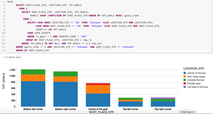
Once we observe that Spanish league has had most goals over the term of this data, we could find top 3 goals locations per shot place from the games in Spain, by writing a more involved query using Window functions in Spark SQL. It would be a stepwise nested query:

top_locs_sp.png
Top 3 goal locations per spot place in Spanish league

We could do time-based analysis as well, e.g. by observing total number of goals over the course of a game (0-90+ minutes), across all games in the five leagues. We could use the “time_bin” column created as part of transformation process earlier, rather than a continuous variable like “time”:

goals_time_bin
Goals per time bin per country/league

Machine Learning

As we saw, doing descriptive analysis on big data (like above) has been made super easy with Spark SQL and Databricks. But what if you’re a Data Scientist who’s looking at the same data to find combinations of on-field playing conditions that lead to “goals”?

We’ll now create a third notebook from that perspective, and see how one could fit a GBT classifier Spark ML model on the game events training dataset. In this case, our binary classification label will be field “is_goal”, and we’ll use a mix of categorical features like “event_type_str”, “event_team”, “shot_place_str”, “location_str”, “assist_method_str”, “situation_str” and “country_code”.

ml_imports
Spark ML imports for the use case

Then the following three-step process is required to convert our categorical feature columns to a single binary vector:

ml_pre-transforms
Spark ML pre-modeling transformations

Finally we’ll create a Spark ML Pipeline using the above transformers and the GBT classifier. We’ll divide the game events data into training and test datasets, and fit the pipeline to the former.

ml_modeling
Create Spark ML pipeline and fit over training data

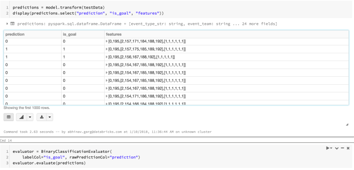
Now we can validate our classification model by running inference on test dataset. We could compare the predicted label with actual label one by one, but that could be a painful process for lots of test data. For scalable model evaluation in this case, we can use BinaryClassificationEvaluator with Area under ROC metric. One could also use the Precision-Recall Curve as evaluation metric. If it was a multi-classification problem, we could’ve used the MulticlassClassificationEvaluator.

ml_evaluate_model
Validate Spark ML model

Conclusion

Above end-to-end data pipeline showcases how different sets of users i.e. Data Engineers, Data Analysts and Data Scientists could work together to find hidden value in big data from any sports.

But this is just the first step. A Sports or Media organization could do more by running model-based inference on real-time streaming data processed using Structured Streaming, in order to provide targeted content to its users. And then there are many other ways to combine different Spark/Databricks technologies, to solve different big data problems in Sport and Media industries.

Try Databricks on AWS or Azure Databricks today.

Monitoring with Telegraf and Cloudwatch

There’re myriad options out there to help monitor applications in real-time, and take preventive/corrective actions and/or notify operations teams. Attributes of interest could be anything from system APU utilization, to memory consumption, to application functional metrics. Any such system should have components playing these roles:

  • Metric Collector
  • Metric Storage
  • Exception Analyzer/Detector
  • Exception Notifier/Alerter

There’re products which do one or more of above – StatsD, FluentD, Elasticsearch, InfluxDB, Grafana, Hipchat, Slack, Alerta and many-many more. You could plug n’ play most of those with one another. DevOps teams are expected to prototype, assess and choose what works best. I’m going to discuss one such bag of products, which is easy to setup, and could be used if your apps are on-premises or in cloud:

  • Telegraf – Metric Collector
  • AWS Cloudwatch Metrics – Metric Storage
  • AWS Cloudwatch Alarms – Exception Analyzer
  • Hipchat/Slack – Exception Notifier

Setup looks like this for a autoscaling Spring Boot app on AWS:

Monitoring with Telegraf

Telegraf is a agent-styled process written in Go, which can collection different metrics using configured plugins. There’re input plugins to collect data, processor plugins to transform collected data, and output plugins to send transformed data to a metric storage. Architecture is very much similar to how LogstashFlume or almost any other collector works. Since our application is deployed on AWS, a configured Cloudwatch agent is already collecting metrics like CPU Utilization, Disk & Network Operations, Load Balancer healthy host count etc. AWS doesn’t measure EC2 memory usage or Disk utilization by default, so we use Telegraf for that purpose and more:

And then Cloudwatch output plugin is configured to send all data to AWS Cloudwatch. A Telegraf agent runs on each EC2 instance of our Autoscaling group – which could be configured as part of a custom AMI, or setup as part of a Cloudformation template. A sample Telegraf configuration looks like this. This is how we configured it for Jolokia and Procstat specifically (as collectors.conf at /etc/telegraf/telegraf.d/):

[[inputs.jolokia]]
 context = "/manage/jolokia/"
 name_prefix = "my_"
 fielddrop = ["*committed", "*init"]
[[inputs.jolokia.servers]]
 host = "127.0.0.1"
 port = "8080"
[[inputs.jolokia.metrics]]
 name = "heap_memory_usage"
 mbean = "java.lang:type=Memory"
 attribute = "HeapMemoryUsage,NonHeapMemoryUsage"
[[inputs.jolokia.metrics]]
 name = "thread_count"
 mbean = "java.lang:type=Threading"
 attribute = "ThreadCount,DaemonThreadCount"
[[inputs.jolokia.metrics]]
 name = "garbage_collection"
 mbean = "java.lang:type=GarbageCollector,*"
 attribute = "CollectionCount,CollectionTime"
[[inputs.jolokia.metrics]]
 name = "class_count"
 mbean = "java.lang:type=ClassLoading"
 attribute = "LoadedClassCount"
[[inputs.jolokia.metrics]]
 name = "metaspace"
 mbean = "java.lang:type=MemoryPool,name=Metaspace"
 attribute = "Usage"
[[inputs.procstat]]
 name_prefix = "my_"
 pattern = "my-xyz-boot.jar"
 fieldpass = ["pid"]

And that’s what Cloudwatch output configuration looks like (as metricstorage.conf at /etc/telegraf/telegraf.d/):

[global_tags]
 InstanceId = "i-xxxxxyyyyyzzzzzzz"
 VPC="myvpc"
 StackName="my-xyz-stack"
[[outputs.cloudwatch]]
 region = "us-east-1"
 namespace = "MY/XYZ"
 namepass = [ "my_*" ]
 tagexclude = [ "host" ]
[[outputs.cloudwatch]]
 region = "us-east-1"
 namespace = "MY/XYZ"
 namepass = [ "my_*" ]
 tagexclude = [ "host", "InstanceId" ]

Of course, one could play around with different options that each plugin provides. It’s recommended to specify your own namespace for Cloudwatch metric storage, and configure the tags which would end up as dimensions for categorization.

Telegraf is a effective data collector and has got a great plugin support, but after all it’s another piece of software to run and manage. There’s a bit-invasive alternative to post your JVM and other functional metrics to Cloudwatch, if you’ve a Actuator-enabled Spring Boot application. Simply import the following libraries through Maven or Gradle:

// Gradle example 
compile group: 'com.ryantenney.metrics', name: 'metrics-spring', version: '3.1.3'
compile group: 'com.damick', name: 'dropwizard-metrics-cloudwatch', version: '0.2.0'
compile group: 'io.dropwizard.metrics', name: 'metrics-jvm', version: '3.1.0'

And then, configure a metrics publisher/exporter, which uses DropWizard integration with Spring Boot Actuator under the hood:

...
...
import org.springframework.context.annotation.Configuration;

import com.amazonaws.services.cloudwatch.AmazonCloudWatchAsync;
import com.codahale.metrics.Metric;
import com.codahale.metrics.MetricRegistry;
import com.codahale.metrics.MetricSet;
import com.codahale.metrics.jvm.GarbageCollectorMetricSet;
import com.codahale.metrics.jvm.MemoryUsageGaugeSet;
import com.codahale.metrics.jvm.ThreadStatesGaugeSet;
import com.damick.dropwizard.metrics.cloudwatch.CloudWatchMachineDimensionReporter;
import com.damick.dropwizard.metrics.cloudwatch.CloudWatchReporterFactory;
import com.ryantenney.metrics.spring.config.annotation.EnableMetrics;
import com.ryantenney.metrics.spring.config.annotation.MetricsConfigurerAdapter;

@Configuration
@EnableMetrics
public class CloudWatchMetricsPublisher extends MetricsConfigurerAdapter {

 @Inject
 private AmazonCloudWatchAsync amazonCloudWatchAsyncClient;

 @Override
 public void configureReporters(MetricRegistry metricRegistry) {

    MetricSet jvmMetrics = new MetricSet() {

       @Override
       public Map<String, Metric> getMetrics() {
          Map<String, Metric> metrics = new HashMap<String, Metric>();
          metrics.put("gc", new GarbageCollectorMetricSet());
          metrics.put("memory-usage", new MemoryUsageGaugeSet());
          metrics.put("threads", new ThreadStatesGaugeSet());

          return metrics;
       }
    };
    metricRegistry.registerAll(jvmMetrics);

    CloudWatchReporterFactory reporterFactory = new CloudWatchReporterFactory();
    reporterFactory.setClient(amazonCloudWatchAsyncClient);
    reporterFactory.setNamespace("MY/XYZ");

    CloudWatchMachineDimensionReporter scheduledCloudWatchReporter = (CloudWatchMachineDimensionReporter) reporterFactory
    .build(metricRegistry);

    registerReporter(scheduledCloudWatchReporter).start(1, TimeUnit.MINUTES);
 }
}

Once available in Cloudwatch, metrics data could be visualized using pre-built graphs and tables. Cloudwatch visualization capabilities can’t be compared with those of Grafana or Kibana, but they are sufficient for a lot of needs. That’s only half of what we want though. To complete the monitoring lifecycle, we need a exception detection mechanism and notify people accordingly. Enter Cloudwatch Alarms, which could be configured to monitor a metric, define a breach point, and send a notification via AWS SNS. SNS is a pub-sub service which could:

Most of the alerting products like Hipchat, Slack, Alerta etc. provide HTTP Webhooks, which could either be invoked directly via HTTP(S) subscription to SNS, or a Lambda could act as a mediator to pre-process the Cloudwatch alarm notification. Some great examples are:

Now, this is what a Cloudwatch alarm for JVM heap usage looks like in Cloudformation:

 "JVMHeapMemoryUsageAlarm": {
 "Type": "AWS::CloudWatch::Alarm",
 "Properties": {
 "ActionsEnabled": "true",
 "AlarmName": "Autoscaling-EC2-HighJVMHeapMemoryUsage",
 "AlarmDescription": "High JVM Heap Memory for Autoscaling-EC2 - My-XYZ",
 "Namespace": "MY/XYZ",
 "MetricName": "my_jolokia_heap_memory_usage_HeapMemoryUsage_used",
 "Dimensions": [{
       "Name": "StackName",
       "Value": {
          "Ref": "AWS::StackName"
       }
    }, {
       "Name": "VPC",
       "Value": "myvpc"
    }, {
       "Name": "jolokia_host",
       "Value": "127.0.0.1"
    }, {
       "Name": "jolokia_port",
       "Value": "8080"
    }
 ],
 "Statistic": "Maximum",
 "Period": "60",
 "EvaluationPeriods": "1",
 "Threshold": 2000000000,
 "ComparisonOperator": "GreaterThanOrEqualToThreshold",
 "AlarmActions": [{
    "Ref": "MyNotificationSNSTopic"
 }]
 }
}

Above alarm will trigger as soon as JVM heap reaches 2GB on any of the EC2 instances in Autoscaling group. Another alarm for Procstat generated metric looks like:

 "SvcProcessMonitorAlarm": {
 "Type": "AWS::CloudWatch::Alarm",
 "Properties": {
 "ActionsEnabled": "true",
 "AlarmName": "Autoscaling-EC2-JavaProcessAvailability",
 "AlarmDescription": "My XYZ Service is down for Autoscaling-EC2 - My-XYZ",
 "Namespace": "MY/XYZ",
 "MetricName": "my_procstat_pid",
 "Dimensions": [{
       "Name": "StackName",
       "Value": {
          "Ref": "AWS::StackName"
       }
    }, {
       "Name": "VPC",
       "Value": "myvpc"
    }, {
       "Name": "pattern",
       "Value": "my-xyz-boot.jar"
    }, {
       "Name": "process_name",
       "Value": "java"
    }
 ],
 "Statistic": "SampleCount",
 "Period": "60",
 "EvaluationPeriods": "1",
 "Threshold": "3",
 "ComparisonOperator": "LessThanThreshold",
 "AlarmActions": [{
    "Ref": "MyNotificationSNSTopic"
 }],
 "InsufficientDataActions": [{
    "Ref": "MyNotificationSNSTopic"
 }]
 }
 }

Above alarm will trigger as soon as Java process goes down on any of the EC2 instances (3) in Autoscaling group. If you’ve alarms for standard metrics – “GroupInServiceInstances” for Autoscaling group, and/or “UnHealthyHostCount” for Load Balancer, those will trigger a bit later than the Procstat one.

Above discussion was more around sending timely notifications in case of exceptional system situations. We can also create up/down policies depending on certain metric data – like increasing or decreasing number of instances automatically based on CPU Utilization. One could go a step further and write a custom application, which subscribes to Alarm SNS topic via HTTP(S) endpoint, and take advanced correction/preventive actions specific to an application. Possibilities are endless with the plug n’ play architecture.

Spring Boot (or Node.js, Django etc.) with Websocket on AWS

Please read on if you’re trying to implement a Spring Boot (or Node.js, Django etc.) Websocket-enabled application on AWS. I’ll keep this brief, covering only the high-level design of how multiple nodes of an AWS-based application cluster get notified of events, and in turn notify connected TCP clients. I’ll not be discussing how client connections to application cluster be maintained. For that, some good folks have already shared extensive information, like:

And if you’re still thinking about whether to use long-polling or Websocket for your interactive application, these might help sway it one way or the other:

Most of our services are created using Spring Boot, though we also use Node.js to a good extent. When it came to design a interactive financial order blotter with interactivity across user sessions, Spring Boot’s support for Websocket clinched the deal. Spring Boot supports Websocket using a Simple in-memory broker, and a full-featured broker for a clustered scenario (which is what we’re going for). Latter approach decouples message passing using a MQ broker like ActiveMQ, RabbitMQ etc. and works amazingly, that allows multiple nodes of a service to provide near real-time updates to connected clients, based on actions from the same group of clients – which is what a order blotter’s selling point is. For more information on how it’s enabled, please refer:

High-level glimpse of how this could be realized on AWS:

Websocket_MQBroker
Autoscaling app cluster with ActiveMQ network of brokers

It looks simple, but despite its many advantages there’re a few issues with this approach, specially when implementing on AWS:

  • MQ broker cluster is another piece of infrastructure to manage, monitor and upgrade continuously
  • Data replication and failover for DR scenario is not straightforward (required continuous back-up of EBS volumes, and then creating new EC2 instance with backed-up volume)
  • Broker network configuration can’t be static (again considering DR/Failover), and maintaining it dynamically is cumbersome – Though there’s a solution in case of RabbitMQ

There’re couple of great alternatives, while using the Simple in-memory broker feature of Spring Boot. And both options depend on AWS managed highly-available messaging services – SNS (pub-sub) and SQS (point-to-point).

Option 1 – Use SNS and SQS with tight coupling

Websocket_SQS-SNS
Autoscaling app cluster with SNS and SQS

In this approach, we’ve replaced the full-featured MQ broker with SNS and SQS. The high-level workflow is:

  • Create a SNS topic, where each service node could send events to (to enable Websocket communication with connected clients)
  • Create a node-specific SQS queue at application boot time, if doesn’t exist already (based on EC2 hostname/private IP), subscribing to the SNS topic
  • User A performs some action on service node A
  • Node A sends action event to SNS topic, and updates UI data for User A and other connected clients to that node via in-memory broker
  • SNS topic publishes action event to Nodes B and C, via respective SQS queues
  • Nodes B and C receive action event from respective SQS queues, and update UI data for respective connected clients via in-memory broker

If the service stack is Autoscaling or the nodes are ephemeral in some other manner, a process to clean-up unused SQS queues is required. A Lambda function, scheduled using Cloudwatch events works perfectly.

Option 2  – Use SNS and SQS with relatively-loose coupling

Websocket_SQS-SNS-DynamoDB
Autoscaling app cluster with DynamoDB, Lambda, SNS and SQS

In this architecture, application is not responsible to send an event to SNS directly. DynamoDB streams and Lambda function take care of that. If you’re already using or planning to use DynamoDB for persistence, this is a great option. The high-level workflow (with highlighted differences) is:

  • Enable stream(s) for DynamoDB table(s) of interest
  • Create a Filter Lambda function, which receives action events from DynamoDB stream(s)
  • Create a SNS topic, which could receive action events from Filter Lambda function
  • Create a node-specific SQS queue at application boot time, if doesn’t exist already (based on EC2 hostname/private IP), subscribing to the SNS topic
  • User A performs some action on service node A
  • Node A modifies data in DynamoDB, and updates UI data for User A and other connected clients to that node via in-memory broker
  • DynamoDB stream sends action event to Filter Lambda function, which can be used to filter events for Websocket communication
  • Filter Lambda sends action event to SNS topic
  • SNS topic publishes action event to Nodes B and C, via respective SQS queues
  • Nodes B and C receive action event from respective SQS queues, and update UI data for respective connected clients via in-memory broker

Both of these options help mitigate challenges with full-featured broker approach, but the downside is that you lock-in to cloud provider managed services. Go-ahead depends on architecture guidelines at one’s place.

These alternatives are not for Spring Boot services only. These would work well with a clustered Node.js or Django Websocket-enabled application as well. Please do comment if you have used so, or could think of other possible design options.

Search Platform using Elasticsearch (on AWS)

Apache Lucene is a high performance, cross-platform search engine library, which has gained immense support in enterprises looking to build firm-wide, customer-facing search platforms. And it does owe good share of its popularity to Apache Solr and Elasticsearch, that are matured search products built on top of Lucene. We chose Elasticsearch 2.3.3 (5.0 is the current version at time of writing), to build our multi-entity search platform for a financial services firm.

All our applications and data platforms are housed in AWS VPCs. We decided to implement our own cluster on EC2 rather than using AWS Elasticsearch, with main reasons being: AWS Elasticsearch doesn’t provide data encryption using AWS KMS yet (at least at time of writing this);  AWS has been generally behind on adding latest Elasticsearch versions; and we wanted full freedom in maintaining our own cluster with choice of security groups, plugins, monitoring etc. Without going into details of infrastructure, I’ll just mention the major plugins we are using:

  • EC2-Discovery for unicast discovery (AWS doesn’t support multicast out of box)
  • Kopf for web-based administration
  • Head for web-based administration
  • SQL for data analysis
  • Read-only to control maintenance actions (alternative to using Nginx as proxy)

elasticsearch-cluster

Our indexing and query services have been implemented in Java (using Spring Boot), and we use Elasticsearch’s Java API (Transport Client) to connect to the cluster. We don’t use Spring Data Elasticsearch, as it also lags behind in version upgrades mostly. Now, moving to what we want to focus on in this blog: how to implement a search service for data stored in Elasticsearch.

First and most important component that impacts data indexing and search in Elasticsearch is an Analyzer. Analysis is the process of converting text, like a product description, or a person name into tokens or terms which are added to the inverted index for searching. Analysis is performed by the analyzer which can be either a built-in or custom. There’re three sub-parts to an analyzer, and they process all incoming text in this order:

  • Character Filter – Used to preprocess text before indexing/searching, like stripping HTML markup
  • Tokenizer – Main component which produces tokens from incoming text
  • Token Filter – Can modify, delete or add tokens to stream of tokens from tokenizer

For our product and person search services (90% of our search functionality), we created custom edgeNGram based token filters, and analyzers using those token filters. A edgeNGram token filter is similar to a nGram token filter, except that it only keeps nGrams which start at the beginning of tokens produced by a tokenizer. The analysis settings for such an index look like:

{
  "settings": {
    "index": {
      ...
    },
    "analysis": {
      "filter": {
        "autocomplete_filter": {
	  "type": "edgeNGram",
	  "min_gram": "1",
	  "max_gram": "10"
	},
	"autocomplete_phrase_filter": {
	  "type": "edgeNGram",
	  "min_gram": "1",
	  "max_gram": "20"
	}
      },
      "analyzer": {
	"keyword_analyzer": {
	  "type": "custom",
	  "filter": [
	    "asciifolding","lowercase"
	  ],
	  "tokenizer": "keyword"
	},
	"autocomplete_analyzer": {
	  "type": "custom",
	  "filter": [
	    "standard","lowercase","stop","autocomplete_filter"
	  ],
	  "tokenizer": "standard"
	},
	"autocomplete_phrase_analyzer": {
	  "filter": [
	    "standard","lowercase","autocomplete_phrase_filter"
	  ],
	  "type": "custom",
	  "tokenizer": "keyword"
        }
      }
    }
  }
}

Now we apply these analyzers to field mappings in the index. In a elaborate search platform, where one needs ability to search a field in different ways, it’s fruitful to store multiple versions of such a field, often using different analyzers during indexing and searching. That way, one could use more relevant version for a given scenario. For e.g.:

{
  "settings": {
    "index": {
      ...
    },
    "analysis": {
     ...
    }
  },
  "mappings": {
    "product": {
      "dynamic": "strict",
      "_all": {
	"enabled": false
      },
      "properties": {
        ...
        ...
	"productTypeCode": {
	  "type": "string",
	  "norms": {
	    "enabled": false
	  },
	  "analyzer": "keyword_analyzer"
	},
        "productName": {
	  "type": "string",
	  "term_vector": "with_positions_offsets",
	  "analyzer": "english",
	  "fields": {
	    "autocomplete_exact": {
	      "type": "string",
	      "norms": {
		"enabled": false
	      },
	      "analyzer": "keyword_analyzer"
	    },
	    "autocomplete_phrase": {
	      "type": "string",
	      "norms": {
		"enabled": false
	      },
	      "analyzer": "autocomplete_phrase_analyzer",
	      "search_analyzer": "keyword_analyzer"
	    },
	    "autocomplete_startswith": {
	      "type": "string",
	      "norms": {
	        "enabled": false
	      },
	      "analyzer": "autocomplete_analyzer",
	      "search_analyzer": "standard"
	    },
	    "autocomplete_token": {
	      "type": "string",
	      "norms": {
		"enabled": false
	      },
	      "index_options": "docs",
	      "analyzer": "standard"
	    },
	    "raw": {
	      "type": "string",
	      "index": "not_analyzed"
	    }
	  }
	}
        ...
        ...
      }
    }
  }
}

What’s worth noting above is how custom analyzers have been used along with built-in analyzers to map different versions of productName (and other fields like that). This is how different versions could be used during searching:

  • productName.autocomplete_exact – to match stored documents that are exactly equal to full queried text (case-insensitive) – Query against “intel corp” will match “Intel Corp“, and not “Intel Corporation“.
  • productName.autocomplete_phrase – to match stored documents that start with full queried text (case-insensitive) – Query against “intel corp” will match both “Intel Corp” and “Intel Corporation“.
  • productName.autocomplete_token – to match stored documents that have exact tokens as full exact tokens in queried text (case insensitive) – Query against “intel corp” will match not just “intel” products, but also “Microsoft Corp” or any other product with “corp“, but won’t match “Microsoft Corporation” or like.
  • productName.autocomplete_startswith – to match stored documents that have tokens that start with tokens in queried text  (case insensitive) – Query against “intel corp” will match not just “intel” products, but also “Microsoft Corp“, “Microsoft Corporation“, “Intellisat” etc.

We use combinations of multiple fields in Elasticsearch queries to order search results (most relevant to least relevant). Elasticsearch Bool Query can be used to construct such compound/combinational queries, with different boost values set for sub-queries to get desired result order (default ordering by descending order of _score).

GET product/_search?search_type=dfs_query_then_fetch
{
  "query": {
    "bool": {
      "should": [
        {
          "constant_score": {
            "query": {
              "match": {
                "productName.autocomplete_exact": "intel corp"
              }
            },
            "boost": 300
          }
        },
        {
          "constant_score": {
            "query": {
              "match": {
                "productName.autocomplete_phrase": "intel corp"
              }
            },
            "boost": 200
          }
        },
        {
          "more_like_this": {
            "fields": ["productName.autocomplete_token"],
            "like": "intel corp",
            "min_term_freq": 1,
            "min_doc_freq": 1,
            "max_query_terms": 10,
            "minimum_should_match": 1,
            "boost": 100
          }
        },
        {
          "constant_score": {
            "query": {
              "match": {
                "productName.autocomplete_startswith": "intel corp"
              }
            },
            "boost": 10
          }
        }
      ],
      "minimum_should_match": 1
    }
  }
}

The above Bool query is composed of Constant Score and More Like This type of queries, which work for us. One should look to replace these sub-queries with appropriate query types, depending on desired search results.

Sometimes, the requirement is to search text in more than one field, with each field stored as multi-fields. For e.g. in our case, user wanted to search in both productName and productDesc fields. In such cases, one could use Dis Max compound query to produce a union of Bool sub-queries (one Bool sub-query per multi-fields field).

GET product/_search?search_type=dfs_query_then_fetch
{
  "query": {
    "dis_max": {
      "queries": [
        {
          "bool": {
            "should": [
              {
                "constant_score": {
                  "query": {
                    "match": {
                      "productName.autocomplete_exact": "intel corp"
                    }
                  },
                  "boost": 300
                }
              },
              {
                "constant_score": {
                  "query": {
                    "match": {
                      "productName.autocomplete_phrase": "intel corp"
                    }
                  },
                  "boost": 200
                }
              },
              {
                "more_like_this": {
                  "fields": ["productName.autocomplete_token"],
                  "like": "intel corp",
                  "min_term_freq": 1,
                  "min_doc_freq": 1,
                  "max_query_terms": 10,
                  "minimum_should_match": 1,
                  "boost": 100
                }
              },
              {
                "constant_score": {
                  "query": {
                    "match": {
                      "productName.autocomplete_startswith": "intel corp"
                    }
                  },
                  "boost": 10
                }
              }
            ],
            "minimum_should_match": 1
          }
        },
        {
          "bool": {
            "should": [
              {
                "constant_score": {
                  "query": {
                    "match": {
                      "productDesc.autocomplete_exact": "intel corp"
                    }
                  },
                  "boost": 300
                }
              },
              {
                "constant_score": {
                  "query": {
                    "match": {
                      "productDesc.autocomplete_phrase": "intel corp"
                    }
                  },
                  "boost": 200
                }
              },
              {
                "more_like_this": {
                  "fields": ["productDesc.autocomplete_token"],
                  "like": "intel corp",
                  "min_term_freq": 1,
                  "min_doc_freq": 1,
                  "max_query_terms": 10,
                  "minimum_should_match": 1,
                  "boost": 100
                }
              },
              {
                "constant_score": {
                  "query": {
                    "match": {
                      "productDesc.autocomplete_startswith": "intel corp"
                    }
                  },
                  "boost": 10
                }
              }
            ],
            "minimum_should_match": 1
          }
        }      
      ]
    }
  }
}

Dis max query generates the union of documents produced by its subqueries, and that scores each document with the maximum score for that document as produced by any subquery, plus a tie breaking increment for any additional matching subqueries.

Here we have discussed just the basic search elements. Elasticsearch provides many other constructs, using which one could filter, rescore (second level of scoring after first search), sort (sort on fields other than on _score) documents, or even use scripting to customize most of these operations. All of these features are quite intuitive to use with Elasticsearch, as we’ve experienced building out our search platform.

Hope you found this article a bit useful. All feedback is welcome.

Automated MongoDB Cluster Backup on AWS S3

If you want a true copy of your MongoDB cluster data in case of data corruption, accidental deletion or disaster recovery, you’ll want to back it up reliably. Automated backup of a MongoDB cluster (with multiple shards) gets a bit complex, because any replica-set stores only one shard at a time, and relevant product utilities dump/export data only from one node at a time. Thus we need to build a custom mechanism to backup all shards simultaneously.

If your MongoDB cluster is setup on AWS, best possible place to store regular backups is S3. And even if the cluster is on-premises, S3 is still a wonderful option (Similar options exist for Azure, Rackspace etc.). Few things to note:

  • You’ll need appropriate permissions to relevant S3 bucket, to store your regular backups.
  • If your MongoDB cluster is on AWS EC2 nodes, it’ll most probably assume a IAM role to interact with other AWS services. In that case, S3 bucket permissions should be granted to the role.
  • If your MongoDB cluster is not on AWS, S3 bucket permissions should be granted to a specific IAM user (better to create a specific backup user). You should have the access credentials for that user (AWS_ACCESS_KEY_ID and AWS_SECRET_ACCESS_KEY).
  • Backup of each MongoDB shard should be taken from one of the secondary nodes of related replica-set. This is to avoid impacting the primary node during backup.
  • To avoid taking duplicate backups on multiple secondary nodes of a replica-set, backup script should run on primary node of that replica-set and connect to one of the secondaries.
  • Each replica-set’s backup node (one of the secondaries) should be locked against any writes during the operation, to avoid reading in-flight writes. It should be unlocked after the backup is complete.
  • You could create a cron job to automate periodic execution of the backup script. If you’re using DevOps to provision your cluster, cron job setup can be done there. We’re using this approach (AWS Cloudformation), to avoid any manual setup.
  • If you’ve a self-healing cluster (like AWS Autoscaling in our case), backup script should be configured to run on all nodes in the cluster. In such a case, script should be intelligent enough to identify the shard and type of node (primary/secondary).

Now the intelligent script:

#!/usr/bin/env bash

export AWS_DEFAULT_REGION=us-east-1

## Provide AWS access credentials if not running on EC2, 
## and relevant IAM role is not assumed
# export AWS_ACCESS_KEY_ID=xxx
# export AWS_SECRET_ACCESS_KEY=yyy

## AWS S3 bucket name for backups
bucket=mybucket

## Create this folder beforehand on all cluster nodes
cd /backup

## Check if the cluster node is a replica-set primary
mongo --eval "printjson(db.isMaster())" > ismaster.txt
ismaster=`cat ismaster.txt | grep ismaster | awk -F'[:]' '{print $2}' | 
          cut -d "," -f-1 | sed 's/ //g'`
echo "master = $ismaster"

if [ "$ismaster" == "true" ]; then
   ## It's a replica-set primary, get the stored shard's name
   shardname=`cat ismaster.txt | grep "setName" | awk -F'[:]' 
             '{print $2}' | grep shard | cut -d"-" -f-1 
             | sed 's/\"//g' | sed 's/ //g'`
   echo "Shard is $shardname"
 
   ## Create a time-stamped backup directory on current primary node
   NOW=$(TZ=":US/Eastern" date +"%m%d%Y_%H%M")
   snapshotdir=$shardname-$NOW
   echo "Creating folder $snapshotdir"
   mkdir $snapshotdir
 
   ## Get the IP address of this primary node
   primary=`cat ismaster.txt | grep primary | awk -F'[:]' '{print $2}' 
           | sed 's/\"//g' | sed 's/ //g'`
   echo "Primary node is $primary"
 
   ## Connect to one of the secondaries to take the backup
   cat ismaster.txt 
       | sed -n '/hosts/{:start /]/!{N;b start};/:27017/p}' 
       | grep :27017 | awk '{print $1}' | cut -d "," -f-1 
       | sed 's/\"//g' 
       | (while read hostipport; do
            hostip=`echo $hostipport | cut -d":" -f-1`
            echo "Current node is $hostip"
 
            ## Check if IP address belongs to a secondary node
            if [ "$hostip" != "$primary" ]; then
              ## Lock the secondary node against any writes
              echo "Locking the secondary $hostip"
              mongo --host $hostip --port 27017 --eval 
                    "printjson(db.fsyncLock())"
 
              ## Take the backup from secondary node, 
              ## into the above created directory
              echo "Taking backup using mongodump connecting 
                    to $hostip"
              mongodump --host $hostip --port 27017 --out 
                        $snapshotdir
 
              ## Unlock the secondary node, so that it could 
              ## resume replicating data from primary
              echo "Unlocking the secondary $hostip"
              mongo --host $hostip --port 27017 --eval 
                    "printjson(db.fsyncUnlock())"
 
              ## Sync/copy the backup to S3 bucket, 
              ## in shard specific folder
              echo "Syncing snapshot data to S3"
              aws s3 sync $snapshotdir 
                  s3://$bucket/mongo-backup/$shardname/$NOW/
 
              ## Remove the backup from current node, 
              ## as it's not required now
              echo "Removing snapshot dir and temp files"
              rm -rf $snapshotdir
              rm ismaster.txt
 
              ## Break from here, so that backup is taken only 
              ## from one secondary at a time
              break
            fi
        done)
else
 ## It's not a primary node, exit
 echo "This node is not a primary, exiting the backup process"
 rm ismaster.txt
fi

echo "Backup script execution is complete"

It’s not perfect, but it works for our multi-shard/replica-set MongoDB cluster. We found this less complex than taking AWS EBS snapshots and re-attaching relevant snapshot volumes in a self-healing cluster. We’d explored few other options, so just listing those here:

  1. An oplog based backup – https://github.com/journeyapps/mongo-oplog-backup
  2. https://github.com/micahwedemeyer/automongobackup

Hope you found it a good read.

Overcome cloud challenges – AWS as Example

Technologies of future (Big Data, IoT, Micro-Services etc.) are optimized to run on commodity hardware and tons of computing, storage and memory resources, which don’t come cheap or fast (“provisioning”). That’s where cloud IaaS and PaaS services come to the rescue. These services enable faster time to market (prototyping anyone?), easy scalability, innovation (AWS Lambda, Azure Cognitive Services etc.) and yes, there’s that cost saving too (if architected and used right though).

But with their advantages, the public cloud technologies have got their share of challenges, due to which their adoption has been slow (particularly in sectors like finance, insurance, auto etc.). In this post, I’ll touch on key general challenges with public cloud technology, and some ways to deal with those if you’re planning to or are already working with Amazon Web Services (AWS) cloud.

Solutions to AWS Challenges
Sample Architecture on AWS, indicating useful services to deal with typical challenges
  • Security – Yep, that’s the first thing you’ll hear from a skeptical executive about public cloud adoption. And we can’t fault them for that, given the nature of some of their processes and operations. I’ll list a few mechanisms using which an organization can keep their applications secure in AWS cloud:
    • Security Groups – In my opinion, this is one of the most basic and powerful features of AWS. It’s just like a private firewall around your instance, which you can configure to control what type of data goes in and out, and to/from specific ports/interfaces. And these are stateful, such that responses to inbound traffic can go out no matter what your outbound traffic restrictions are.
    • Access Control Lists (ACLs) – There are network ACLs, which work like Security Groups at the subnet layer. These are also a set of rules, and you can (read should) configure them to allow/deny specific traffic to/from your subnets. These are stateless though, i.e. response traffic must be explicitly configured in allow rules. Then there are S3 ACLs, which you can configure to control access to your S3 buckets and objects. Right combination of Security Groups and ACLs should be utilized when deploying your application(s) to AWS.
    • Identity and Access Management (IAM) – IAM is about authentication and authorization for your AWS resources. Whether it’s a developer accessing AWS console from within your firm, or a EC2 instance accessing DynamoDB etc., IAM manages all of it. Think of it as a Directory Service composed of users & groups, and roles assigned to them. You can configure macro to micro level permissions and policies, allowing or denying particular action(s) on particular resource(s). Right policy configurations can protect your applications/resources from unauthorized access. If required, one can also add Multi-factor authentication for account access, enabled via virtual (your phone) or hardware devices (key fob/display card).
    • Secure Token Service (STS) – STS provides temporary, limited-privilege credentials for your IAM or federated users (like Active Directory users federated using ADFS). It basically generates a short-lived token (configurable time), using which a user could access required AWS resources during that time. The access is terminated once the token expires. STS is a powerful service which should be used to control access to AWS console or resources.
  • Data Privacy – In sensitive environs, like Financial Services, Healthcare, Insurance etc., keeping data secure is a huge deal. And as we’ve seen in recent past, even government services and large internet companies have been victims of data breaches, which leads to loss of trust and clamor for more regulations/laws to protect consumer data. But there’re ways to keep data secure in a public cloud like AWS:
    • SSL/TLS for in-transit data – This is basic stuff, but worth reminding. If you have two applications talking to each other, and both are deployed in a private subnet in a VPC, maybe SSL/TLS can be skipped. But in enterprise world, since cloud infrastructure is mostly realized in a hybrid model, you’ll have on-premises applications talking to cloud-deployed applications, and also business users accessing those applications. In such cases, SSL/TLS becomes mandatory.
    • Key Management Service (KMS) – KMS is a service to generate and store encryption keys, which can be used to encrypt your data at rest, whether it’s stored in S3, RDS or EBS volumes. The keys can be rotated to ensure that your encryption/decryption process is safe in longer run (just like resetting passwords periodically). KMS also provides an audit trail of key usage.
    • Encrypted EBS Volumes – If your data is stored in EBS volumes (self-managed relational database/NoSQL cluster, or a file store etc.), the volumes should be encrypted to keep data secure. The data is encrypted at rest and in transit to/from EC2 instance. A snapshot created from an encrypted volume is also encrypted. Internally, EBS encryption uses KMS managed keys. Encryption is supported for all EBS types, but not all EC2 instance types support encrypted volumes.
    • Hardware Security Module (HSM) – This is a tamper-resistant hardware appliance, that can be used to securely store cryptographic key material. Some organizations have to meet strict regulatory and contractual requirements with respect to data security, and HSM devices can aid in such situations. You’ll need a private subnet in your VPC to house the HSM appliance.
    • Data Governance – This is a general concept, which should be adopted by organizations looking to move to cloud (if not done yet). Data Governance is not just about creating a fat committee, but it’s identifying different tiers of data, which have different degrees of sensitivity and privacy, and to do that continuously. The exercise helps define guidelines around which data can reside in cloud, and which not. If it’s decided to keep sensitive and confidential data on-premises, a hybrid cloud by way of a VPC (VPN-over-IPSec or Direct Connect) can still be realized to keep your application in cloud, that can access on-premises stored data securely (though the in-transit data should be encrypted).
  • Availability – Another area of concern with public clouds has been availability of overall infrastructure and services. Cloud outages were a regular feature in news in the past, leading to downtime for customer applications. Over last couple of years though, major public cloud providers have made considerable improvements to their infrastructure to be able to flaunt availability figures of 99.95% and so. But if you do a rough calculation, even that figure can cause headache for executives. Since cloud service outages are generally location specific, impact to your applications can be avoided through sound architecture decisions:
    • Multi-Region Deployment – Regions in AWS are completely isolated geographic areas, providing high level of fault tolerance. For HA (hot-hot or hot-warm) multi-region deployment, one has to consider replication of different resources across regions. EC2 computing instances can be maintained in a hot/warm state, whereas out-of-box cross-region asynchronous replication can be done for data in S3 or RDS. If you manage your own data layer on EC2, you’ll have to implement your own replication mechanism. Network failover can be achieved using Route 53 routing policies (latency based or failover).
    • Multi-AZ Deployment – Availability Zones (AZ) in AWS are like isolated data centers within a region. And Amazon has been working to continuously increase number of AZs in major regions. Application and Data clusters should be deployed across different AZs in a region to provide redundancy and load balancing. When employing Multi-Region or Multi-AZ architecture, you mitigate against risk of localized regional failures.
    • Utilize DevOps – Automated deployments using configuration management tools/services (AWS OpsWorks, Puppet, Saltstack etc.), along with the power of monitoring triggered actions can help reduce the downtime to a minimum. In addition, DevOps thinking can also help standardize development processes across teams. Thus, it’s imperative to consider DevOps while designing your deployment architecture.
  • Vendor lock-in – One other bottleneck regularly mentioned during cloud strategy discussions is locking-in to features and capabilities of a particular cloud provider. People fear that once they are deep into using AWS or Azure or some other public cloud, it’s hard to change down the line. The hesitation is not without reason, because major cloud providers have been so far poor at interoperability. But there’s light at the end of the tunnel. Some organizations are working to create such standards for future, like DMTF Open Virtualization Format (OVF), OASIS TOSCA etc. But until their adoption, there are other options to avoid lock-in. There’re Openstack based cloud providers to choose from, most popular being Rackspace. Or if you have got your eyes set on one of the big guns, you can look at Pivotal Cloud Foundary as a service management platform to abstract a cloud provider. Same can be achieved to a good extent with any configuration management tool as well (listed above in DevOps).

There are other challenges like Compliance with different industry regulations, skill upgrade of existing teams etc. To address the first, public cloud providers like AWS have made long strides in conforming to various standards and regulations to increase wide adoption. For second, problem of stale skills can be managed by investing in brief-to-thorough training programs. And I’m not talking about break-the-bank programs out there, there are much cheaper online options available with good enough content – like cloudacademy.com, linuxacademy.com etc.

Through this post, I just wanted to highlight a few ways on how to tackle key bottlenecks while moving to AWS. These are definitely not end in themselves, nor are these absolutely full-proof solutions. But these can act like a basic checklist, and one should dig deeper to understand nuances and grey areas before adoption.

Performance Best Practices for MongoDB

MongoDB is a document-oriented NoSQL database, used as data backbone or a polyglot member for many enterprise and internet-targeted systems. It has an extensive querying capability (one of the most thorough in NoSQL realm), and integration is provided by most of popular application development frameworks. There are challenges in terms of flexible scaling, but it’s a great product to work with once you come to terms with some of the nuances (you need patience though).

We’re using MongoDB as an event store in a AWS deployed financial data management application. The application has been optimized for write operations, as we have to maintain structures from data feeds almost throughout the day. There are downstream data consumers, but given defined query patterns, read performance is well within the defined SLA. In this blog, I’ll share some of the key aspects that could help improve write performance of a MongoDB cluster. All of these might not make sense for everyone, but a combination of a few could definitely help. MongoDB version we’re working with is 3.0.

  • Sharding – Sharding is a way to scale-out your data layer. Many in-memory and NoSQL data products support sharded clusters on commodity hardware, and MongoDB is one of those. A shard is a single MongoDB instance or a replica-set, that holds a subset of total data in the cluster. Data is divided on basis of a defined shard key, which is used for routing requests to different shards (by mongos router). A production-grade sharded cluster takes some time to setup and tune to what’s desired, but yields good performance benefits once done right. Since data is stored in parts (shards), multiple parts can be simultaneously written to without much contention. Read operations also get a kick if queries contain the shard key (otherwise those can be slower than non-sharded clusters). Thus, choosing the right shard key becomes the most important decision.

MongoDB App Cluster

  • Storage Engine – Storage engine determines how data will be stored in memory and on disk. There are two main storage engines in MongoDB – WiredTiger and MMAPv1. MMAPv1 was default until version 3.0, and WiredTiger is default in 3.2. Biggest difference between the two is that MMAPv1 has at best collection-level locking for writes, whereas WiredTiger has document level locking (mostly optimistic). Thus, WiredTiger can allow for a more fine-grained concurrency control, and more parallel writes possibly. WiredTiger also comes with data compression on disk, plus has a checkpointing feature to maintain consistency (in addition to default Journaling). If you’re using version 3.0, MMAPv1 could still be good enough given that it’s a tried and tested component and WiredTiger was still fairly new at that point.
  • Write Concern – Write concern allows one to define the degree of acknowledgement indicating success of a write operation. If a system can easily recover write losses without observable impact to users, then it’s possible to do away with acknowledgements altogether, so as to make the write round-trip as fast as possible (Not allowed if Journaling is ON). By default, acknowledgement is required from a standalone instance or primary of a replica set. If one wants strong consistency from a replica set, write concern can be configured to be more than 1 or “majority” to make sure writes have propagated to some replica nodes as well (though it’s done at cost of degraded write performance).
  • Journaling – Journaling is basically write-ahead logging on disk to provide consistency and durability. Any chosen storage engine by default writes more often to the journal than to the data disk.  One can also configure Write Concern with “j” option, which indicates that operation will be acknowledged after it’s written to the journal. That allows for more consistency, but overall performance can take a hit (duration between Journal commits is decreased automatically to compensate though). From a performance perspective, there’re a couple of things one can do with respect to Journaling – 1. Keep journal on a different volume than the data volume to reduce I/O contention, and/or 2. Reduce interval between journal commits (please test this thoroughly, as too less a value can eventually decrease overall write capacity).
  • Bulk Writes – One can write multiple documents in a collection through a single bulk-write operation. Combined with WiredTiger storage engine, this can be a great way to make overall writes faster if it’s possible to chunk multiple writes together. Though if you’ve a e-commerce system, and you need to handle write operations per user transaction, it might not be a great option. Bulk writes can be ordered (serial and fail-fast) or unordered (parallel isolated writes), and the choice depends on specific requirements of a system.

There’re other general and non-intrusive ways to improve overall performance of a MongoDB cluster, like increase memory (to reduce read page faults), use SSD for data volume, or increase disk IOPS (should be employed if cost and infra limits permit). What we’ve covered above are specific MongoDB provided features, which can be played around with, provided there’s appetite.

Hope this was a wee bit helpful.

Amazon (AWS) SQS with Spring Cloud

Amazon Simple Queue Service (SQS) is a HA cloud messaging service, that can be used to decouple parts of a single system, or integrate multiple disparate systems. A SQS queue acts as buffer between a message producer and a consumer, when former’s message generation rate is more than latter’s processing throughput. It also provides durable point-to-point messaging, such that messages are stored in a fail-safe queue, and can be processed once a consumer application comes up after scheduled maintenance or unexpected downtime. For publish-subscribe design pattern, Amazon (AWS) provides another cloud service called Simple Notification Service (SNS).

Integration_with_Amazon_SQS

Above diagram shows a subset of possible producer-consumer scenarios that can utilize SQS.

For developers who use JMS to connect to messaging providers/brokers like ActiveMQ, Websphere MQ, JBoss Messaging etc., they can use Amazon SQS Java Messaging Library to work with SQS. One can use it along with AWS SDK to write JMS 1.1 compliant applications. But for real-world applications, writing directly with AWS provided library can be cumbersome. That’s where Spring Cloud AWS comes to the rescue. In this post, I’ll show how one can use Spring Cloud with Spring Boot to write a SQS message producer and a consumer. Before that, a few important points to note when working with SQS:

  • Maximum payload of a SQS message can be 256 KB. For applications that have need to send more data in a single packet, could use SQS Extended Client Library which utilizes AWS S3 as the message store (with a reference being sent in actual SQS message). Other option is to compress the message before sending over SQS.
  • Messages can be sent synchronously, but received either synchronously or asynchronously (Using AmazonSQSAsyncClient). If required, one can send messages in a separate child thread so as not to block the main thread for SQS IO operation.
  • Messages can be sent or received in batch to increase throughput (10 messages at max in a batch). Please note that maximum payload size limit for a batch message is also 256 KB, so it can only be used for lighter payloads.
  • There can be multiple producer and consumer threads interacting with the same queue, just like any other messaging provider/broker. Multiple consumer threads provide load balancing for message processing.
  • Consumers can poll for messages using long polling and standard polling. It’s recommended to use long polling to avoid too many empty responses (one can configure timeout).
  • Each message producer or consumer needs AWS credentials to work with SQS. AWS provides different implementations of AWSCredentialsProvider for the same. DefaultAWSCredentialsProviderChain is used by default, if no provider is configured specifically.

Now, how to use Spring Cloud with SQS. First of all, below dependencies should be provided in  Maven project’s pom.xml or Gradle’s build file. AWS SDK and other Spring dependencies would be automatically added to the classpath (unless already specified explicitly).

<dependency>
	<groupId>org.springframework.cloud</groupId>
	<artifactId>spring-cloud-aws-autoconfigure</artifactId>
	<version>latest.version</version>
</dependency>
<dependency>
	<groupId>org.springframework.cloud</groupId>
	<artifactId>spring-cloud-aws-messaging</artifactId>
	<version>latest.version</version>
</dependency>

From a configuration perspective, we first need to wire the appropriate AWS SQS client. Assuming  asynchronous interaction with SQS, we will configure a AmazonSQSAsyncClient. There’re a couple of things to note. One, if you’re behind a proxy, you’ll need to specify proxy host and port using ClientConfiguration. Second, DefaultAWSCredentialsProviderChain will look for AWS access key, secret access key and default region in this order – environment variables, system variables, properties file and instance profile (only in EC2). We’ve just overridden the default region below (which is also us-east-1 though).

@Lazy
@Bean(name = "amazonSQS", destroyMethod = "shutdown")
public AmazonSQSAsync amazonSQSClient() {
    AmazonSQSAsyncClient awsSQSAsyncClient;
    if (useProxy.equalsIgnoreCase("Y")) {
	ClientConfiguration clientConfig = new ClientConfiguration();
	clientConfig.setProxyHost("proxy.xyz.com");
	clientConfig.setProxyPort(8085);

	awsSQSAsyncClient = new AmazonSQSAsyncClient(new DefaultAWSCredentialsProviderChain(), clientConfig);
    } else {
	awsSQSAsyncClient = new AmazonSQSAsyncClient(new DefaultAWSCredentialsProviderChain());
    }
		
    awsSQSAsyncClient.setRegion(Region.getRegion(Regions.fromName("us-east-1")));
    return awsSQSAsyncClient;
}

Next we look at configuring a QueueMessagingTemplate, which will be used to send messages to a SQS queue.

@Configuration
public class ProducerAWSSQSConfig {
   ...

   @Bean
   public QueueMessagingTemplate queueMessagingTemplate() {
	return new QueueMessagingTemplate(amazonSQSClient());
   }
   
   @Lazy
   @Bean(name = "amazonSQS", destroyMethod = "shutdown")
   public AmazonSQSAsync amazonSQSClient() {
   ...
}

@Component
public class MessageProducer {

   private QueueMessagingTemplate sqsMsgTemplate;
   ...

   public void sendMessage(String payload) {
      ...
      this.sqsMsgTemplate.convertAndSend("randomQName", payload);
      ...
   }
}

We’re sending a String message, which will be converted using a StringMessageConverter internally. One can also send a complete data object as JSON, if Jackson library is available on classpath (using MappingJackson2MessageConverter).

Finally, we look at configuring a SimpleMessageListenerContainer and QueueMessageHandler, which will be used to create a message listener for SQS queue. Please note that internally Spring Cloud creates a SynchonousQueue based thread pool to listen to different queues and to process received messages using corresponding handlers. Number of core threads for thread pool are 2 * number of queues (or configured listeners), and property “maxNumMsgs” determines the maximum number of threads. Property “waitTimeout” determines the timeout period for long polling (default with Spring Cloud).

public class ConsumerAWSSQSConfig {
   ...

   @Bean
   public SimpleMessageListenerContainer simpleMessageListenerContainer() {
	SimpleMessageListenerContainer msgListenerContainer = simpleMessageListenerContainerFactory().createSimpleMessageListenerContainer();
	msgListenerContainer.setMessageHandler(queueMessageHandler());
	
        return msgListenerContainer;
   }

   @Bean
   public SimpleMessageListenerContainerFactory simpleMessageListenerContainerFactory() {
	SimpleMessageListenerContainerFactory msgListenerContainerFactory = new SimpleMessageListenerContainerFactory();
	msgListenerContainerFactory.setAmazonSqs(amazonSQSClient());
	msgListenerContainerFactory.setDeleteMessageOnException(false);
	msgListenerContainerFactory.setMaxNumberOfMessages(maxNumMsgs);
	msgListenerContainerFactory.setWaitTimeOut(waitTimeout);
	
        return msgListenerContainerFactory;
   }

   @Bean
   public QueueMessageHandler queueMessageHandler() {
	QueueMessageHandlerFactory queueMsgHandlerFactory = new QueueMessageHandlerFactory();
	queueMsgHandlerFactory.setAmazonSqs(amazonSQSClient());
	
        QueueMessageHandler queueMessageHandler = queueMsgHandlerFactory.createQueueMessageHandler();

	return queueMessageHandler;
   }
   
   @Lazy
   @Bean(name = "amazonSQS", destroyMethod = "shutdown")
   public AmazonSQSAsync amazonSQSClient() {
   ...
}
@Component
public class MessageConsumer {
   ...

   @MessageMapping("randomQName")
   public void onRandomQMessage(String payload) {
	doSomething(payload);
   }
}

One can also send custom message attributes (headers) with a SQS message, so as to provide contextual information to the consumer. In addition, there’re important concepts of visibility timeout and delay queues, which should be explored before getting your hands dirty with SQS.

Hope you have fun with Spring Cloud and AWS SQS.

Data analysis with Spark Streaming

Data analysis with Spark Streaming

Apache Spark has more than taken off by now. It’s being used to solve myriad types of data analysis problems, whether it’s a recommendation system for a modern retail store, or a business intelligence platform for a conservative financial asset manager, and many. Apart from its features and performance to reckon with, a big part of Spark’s success was its support for Python, which led to its widespread adoption. And now they’ve added a R package SparkR, which has been a attention grabber for all those R enamored data scientists out there. No doubt it has taken a fair share of limelight from Hadoop Mapreduce.

Apart from the core Spark engine, there’re four add-on modules that make this framework a powerhouse to reckon with:

  • Spark Streaming – to process real-time data streams
  • Spark SQL and Dataframes – to support relational data analysis, and data structures common to R and Python Pandas.
  • Spark MLib – to create machine learning applications
  • Spark GraphX – to solve graph functional problems, like in hierarchies, networks etc.

In this post, we’ll look at a simple data problem, which needs some computation over a continuous stream of US consumer complaints data (Source: Data.gov). We’ll be using Spark Streaming  (Java API) with Apache Flume (a data collector and aggregator) to exemplify real-time data analysis. Flume will be used as a generator of real-time data events (for sake of simplicity, we’re using a finite dataset). Whereas a standalone Spark Streaming program will consume events as they are generated, maintain a rolling count of consumer complaints by type and US state, and store results to a file at a frequency.

Spark_Streaming_with_FlumeIt’s a hypothetical problem, hence you’ll see events being generated from a finite dataset (CSV file of consumer complaint records – many columns removed to keep it simple). Our sample data looks like this:

"Debt collection","Credit card","MA"
"Bank account or service","Checking account","TN"
"Consumer loan","Vehicle loan","FL"
"Bank account or service","Savings account","PA"
"Debt collection","","GA"
"Debt collection","Credit card","FL"
"Debt collection","Medical","DE"
"Credit reporting","","TX"
"Mortgage","Other mortgage","CA"

First we see a basic Flume event generator (with Avro source). It needs a running Flume agent (directions mentioned below). Full source for event generator is available at Flume Client.

// Initialize connection to Flume agent, and the event source file
public void init(String hostname, int port) {
	// Setup the RPC connection
	this.hostname = hostname;
	this.port = port;
	this.client = RpcClientFactory.getDefaultInstance(hostname, port);

	try {
		InputStream inStream = this.getClass().getClassLoader()
				.getResourceAsStream("cons_comp_data.csv");
		Reader in = new InputStreamReader(inStream);
		csvRecords = CSVFormat.DEFAULT.
                             withSkipHeaderRecord(true).parse(in);
	} 
        .......
        .......
}

// Send records from source file as events to flume agent
public void sendDataToFlume() {
	CSVRecord csvRecord = null;
	Iterator csvRecordItr = csvRecords.iterator();
	while (csvRecordItr.hasNext()) {
		try {
			csvRecord = csvRecordItr.next();
			String eventStr = csvRecord.toString();
			System.out.println(eventStr);
			Event event = EventBuilder.withBody(eventStr,
					Charset.forName("UTF-8"));
			client.append(event);
		} 
                .......
                .......
	}
}

Now we take a look at the Spark Streaming program, which processes each event to maintain a rolling count by complaint type and state. At the start, we create a JavaStreamingContext, which is the entry point to a Spark Streaming program, and create a input stream of events using Spark-Flume integration.

SparkConf sparkConf = new SparkConf().setAppName("ConsCompEventStream");

// Create the context and set the checkpoint directory
JavaStreamingContext context = new JavaStreamingContext(sparkConf,
				new Duration(2000));
context.checkpoint(checkpointDir);

// Create the input stream from flume sink
JavaReceiverInputDStream flumeStream = FlumeUtils.createStream(context, h  ost, port);

We are setting a checkpoint folder in JavaStreamingContext, which is used to create Fault tolerant Spark Streaming applications. It allows the application to recover from failures. Please read more at Spark Checkpointing.

Rest of the program processes each Flume event in logical steps:

  • Use map() function to convert incoming stream of events to a JavaDStream. This allows us to convert each Flume event into a processable format.
  • Use mapToPair() function to convert each processable event to a JavaPairDStream of complaint type and US state.
  • Use updateStateByKey() function to maintain a rolling count by complaint type and US state.
  • Use foreachRDD() function to store the rolling count to a file periodically.
// Transform each flume avro event to a processable format
JavaDStream transformedEvents = flumeStream
		.map(new Function<SparkFlumeEvent, String>() {
                  .........
                };

// Map key-value pairs by product and state to count of 1
JavaPairDStream<Tuple2<String, String>, Integer> countOnes = transformedE  vents
		.mapToPair(new PairFunction<String, Tuple2<String, String>,   Integer>() {
                  .........
                };

// Maintain a updated list of counts per product and state
JavaPairDStream<Tuple2<String, String>, List> updatedCounts = countOnes
		.updateStateByKey(new Function2<List, Optional<List>, Optio  nal<List>>() {
                  .........
                };

// Store the updated list of counts in a text file per product and state
updatedCounts.foreachRDD(new Function<JavaPairRDD<Tuple2<String, String>,   List>, Void>() {
                  .........
                };

Full source is available at Spark Flume Stream. It also includes complete information on how to configure and run the Flume agent, as well as how to run this program using a local Spark cluster. The implementation is in Java 1.7, hence the use of anonymous inner classes. It can look a lot concise and prettier if converted to use lambdas with Java 8. I won’t mind a merge request for the same ;-).